Keywords
NLTK; Brown Corpus; WordNet; Sentence similarity; Word order vector;
Word similarity; Automatic Text Summarizer
Introduction
With fastest growing internet facility and technological people
currently trust internet more than a bank locker or private safe.
People are using internet to keep data secret and safe from the
attack of unauthorized personnel. As we know World Wide Web
in 21st century makes revolution in technology field or to be
precise in the Information Technology, and the more revolutions
are waiting to come. To keep this revolution moving on the
Data Mining approach becomes a buzzword in these decades.
In a short-term data mining refers to approach the practice of
examining large pre-existing databases in order to generate new
information [1]. A small field of data mining is text mining. Text
mining, also referred to as text data mining, roughly equivalent to
text analytics, is the process of deriving high-quality information
from text [2]. Text mining redirects to one of the important
applications which is text summarization [3-5].
Text summarization is one of the challenging and important
problems of text mining. It provides several benefits to users.
A vast number of real-life problems can also come to a fruitful
conclusion with text summarization. In this chapter we will give
some idea about text summarizing and its automotive mode. We
will also cover the classification of text summarization. Then we
will discuss about the objectives of our paper. After that, we will cover steps of summarizing process along with brief discussion
about extraction based summarizing technique. At the end of this
chapter we will try to illustrate why we choose this approach for
Bengali Language [6-9].
The extractive summarization process evolves with several
fascinating algorithms. From those algorithms we worked with
the statistical approach and graph-based sentence similarity
approach [10,11].
Statistical Approach
In statistical approach we first initialize the min_cut and max_cut
values. Words that have probabilistic appearance less than min_
cut and more than max_cut will be ignored. The list of stop words
then will also be considered as non-countable. After tokenizing
every word except the stop words, we calculated frequency
of each word. In this situation all the words are mapped using
python’s hash map structure that stores the words as an object.
Then we did calculate the maximum among frequency of words.
Then to figure out the statistical score of words we will use the
formula given below-

Here, Ai is the number of appearances of a certain word obviously
without stop words and M is the maximum number among
frequency of words.
Doing this calculation for each of the sentences we got the
statistical score of each word. After this calculation we have
calculated the total score of a sentence by placing the score of all
the words and for the stop words it the score is null.
The equation of the score o f a sentence can be shown as –

By implementation of this equation once we have the score of all
the sentences, we can give output the sentences with most scored
K sentences at our ease. As we are implanting this algorithm in
Bengali, we need to make a different library of Bengali stop words.
Pre-Processing
Text pre-processing simply illustrates organize texts for further
usage. Pre-Processing is vital pre-requisite while working with
noisy text content like social media, news content crawler and all
that. Pre-processing involves splitting content into valid tokens,
words and symbols, stemming, moving out stop words and parts
of speech tagging. Here we have used the nltk tokenizer with a
slight modification although built for English works smoothly for
Bengali as well [12].
Computation of Word Similarity
Working on the word similarity we have to first illustrate the
WordNet lexicon analysis which is a Bengali lexical knowledge
base that will obviously help for NLP and next we will illustrate
the word similarity procedure [13].
Wordnet lexicon formation
To calculate word similarity between any two Bengali words a
lexicon should be developed. In this we have used the lexicon
developed by (Manjira, Sinha, Tithankar, Anupam). In that lexicon
they constructed a hierarchical conceptual graph. The storage and
organization of their database facilitate computational processing
of the information and efficient searching to retrieve the details
associated with any words [14]. Therefore, it is really a fantastic
resource and tool for NLP analysing in Bengali. It supports query
like DETAILS(X) where X can be any type of node in hierarchy and
SIMILARITY (W1, W2) that returns the similarity between any
two words based on the word’s organization i.e. either they are
synonym, similar, stop word etc. The formation of the lexicon
is pretty simple. The lexicon contains 30 different sections as
30 different roots. Words are also categorized, sub-categorized
using parts of speech. Corresponding each of the category there
are two clusters. The first one contains the synonym of a word
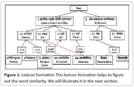
and the other one contains related word [14]. Figure 1 below will
illustrate the lexicon basic formation.
Figure 1: Lexicon formation This lexicon formation helps to figure
out the word similarity. We will illustrate it in the next section.
Word similarity computation
To calculate word similarity based on the lexicon we will measure
the distance between two words. Let us given two words
“Universe” and “Universe”. As both of them are in same cluster
i.e. within the synonym cluster then the similarity is obviously
same. But if we consider another two words “Universe” and
“Astronomer”. Both of them are in different cluster. They are not
synonyms to each other. Instead they are related word to each
other and the distance between those two words are path length
which is 4. As we are calculating similarity then we must have to
choose the words with more similarity i.e. lesser path distance.
However, this method may be less accurate if it is applied to
larger and for more general semantic nets such as WordNet.
For example, let us have the distance between words “Man”
and “Animal” is lesser than the distance between words “Man”
and “Doctor”. Then obviously similarity returns wrong result.
To resolve this issue, we may create categorized word lexicon. If
we create a category called “Human” then put all related words
under this category and another category called “Animal” then
put all the related words under this category we hope task will
be a bit easier and the distance will be a larger such as adding
the real distance with a constant value [15,16]. Therefore, the
depth of word in the hierarchy should be taken into account. In
summary, similarity between words is determined not only by
path lengths but also by depth. We propose that the similarity S
(w1, w2) between words w1 and w2 is a function of path length
and depth as follows:

where l is the shortest path length between W1 and W2, h is the
depth of subsume in the hierarchical semantic nets. We assume
that (3) can be rewritten using two independent functions as:

f1 and f2 are transfer functions of path length and depth,
respectively. We call these information sources of path length
and depth, attributes [17-19].
Transfer function and its characteristics
Transfer functions are those functions that calculate similarities
between words or sentences based on several parameters. The values of an attribute in equation (4) may cover a large range up
to infinity, while the interval of similarity should be finite with
extremes of exactly the same with a value of 1 and no similarity
as 0, then the interval similarity is (0, 1). Direct use of information
sources as a metric of similarity is inappropriate due to it infinite
property. Therefore, it is intuitive that the transfer function
from information sources to semantic similarity is a nonlinear
function. Taking path length as an example, when the path length
decreases to zero, the similarity would monotonically increase
toward the limit 1, while the path length increases infinitely, the
similarity should monotonically decrease to 0. So, to meet these
constraints the transfer function must be a nonlinear function.
The nonlinearity of the transfer function is taken into account in
the derivation of the formula for semantic similarity between two
words [20,21].
Path Length and its Contribution
Considering the path length between any two words w1 and w2
can be determined by one of the following three cases:
1. w1 and w2 are in the same synset.
2. w1 and w2 are not in the same synset, but the synset for w1
and w2 contains one or more common words.
3. w1 and w2 are neither in the same synset nor do their synsets
contain any common words.
Case 1 simply illustrate that both of the words are of same
meaning and hence the path length is 0. For case 2 partially they
share the same feature and hence path length is 1. For case 3,
we will compute the actual path length. Based on the previous
consideration we set f 1(l) (4) to be a monotonically decreasing
function of l:

where, α is a constant. The selection of the function in exponential
form ensures that f 1(l) satisfies the constraint and the value of f
1(l) within the range of 0 and 1.
Effects of Depth Scaling
Words at upper layers of hierarchical semantic nets have more
general concepts and less semantic similarity between words
than words at lower layers. This behavior must be taken into
account in calculating S (w1, w2). We therefore need to scale
down S (w1, w2) for subsuming words at lower layers. As a result,
f2(h)should be monotonically increasing with respect to h. So, f
2 will be:

where,  is a smoothing factor. As
  then the depth of a
word in the semantic nets is not considered. In summary, the
formula for a word similarity measure as:

Where 
are parameters scaling the contribution of shortest path length and depth, respectively. The
optimal values of and ' are dependent on the knowledge base
used and can be determined using a set of word pairs with human
similarity rating. With several calculations it has been seen that the proposed measure of is 0:2 and 0:45 [22].
Semantic Similarity between Sentences
A sentence consists of some words. It would be easier to calculate
things if we represent a sentence as a vector of words. Given two
sentence T1 and T2, a joint word set is formed:

The joint word set T contains all the distinct word set. Since
inflectional morphology may cause a word to appear in a
sentence with a different form that conveys a specific meaning
for a specific context, we consider them as different words. For
example, boy and boys considered as two different words and all
will be included in the word set [23-25].
Here in T the algorithm removes duplicate words skipping the
stop words. The vector derived from the joint word set is called
the lexical semantic vector, denoted by S. Each entry of the
semantic vector corresponds to a word in the joint word set, so
the dimension equals the number of words in the joint word set.
The value of an entry of the lexical semantic vector, Si (i=1, 2,….n)
is determined by the semantic similarity of the corresponding
word to a word in the sentence. Take T1 as an example:
Case 1: If Wi appears in the sentence, Si is set 1
Case 2: If Wi is not contained in T1, a semantic similarity score
is computed between Wi and each word in the sentence T1.
Thus, the most similar word in T1 to Wi is that with the highest
similarity score γ If γ exceeds a present threshold, then S I = γ otherwise, S I = 0. The reason for the introduction of the threshold
is twofold. First, since we use the word Similarity of distinct words
(different words), the maximum similarity scores may be very low,
indicating that the words are highly dissimilar. In this case, we
would not want to introduce such noise to the semantic vector.
Second, classical word matching methods (1) can be unified into
the proposed method by simply setting the threshold equal to
one. Unlike classical methods, we also keep all function words.
This is because function words carry syntactic information that
cannot be ignored if a text is very short (e.g. sentence length).
Although function words are retained in the joint word set, they
contribute less to the meaning of a sentence than other words.
Furthermore, different words contribute toward the meaning
of a sentence to differing degrees. Thus, a scheme is needed to
weight each word. We weight the significance of a word using
its information content. It has been shown that words that occur
with a higher frequency (in a corpus) contain less information
than those that occur with lower frequencies [26]. The value of
an entry of a semantic vector is:

where, Wi is a word of joint set, is its associated word in
sentence. The use of I (Wi) and
 allows the concerned
two words to contribute to the similarity based on their individual
information contents. Here wi and
 can be calculated as
follows:

Where, n = number of times word w in corpus N = number of
words in the corpus, So, I ∈ [0,1]. The semantic similarity between
two sentences is defined as the cosine coefficient between the
two vectors:

It is worth mentioning that the method does not currently
conduct word sense disambiguation for poly-serous words. This
is based on the following consideration: First we wanted to our
model to be as simple as possible and not too demanding in
terms of computing resources. The integration of word sense
disambiguation would scale up the model complexity. Second
existing sentences similarity methods do not have included word
sense [27].
Word Order Similarity between
Sentences
The word order similarity attempts to correct for the fact that
sentences with the same words can have radically different
meanings. This is done by computing the word order vector for
each sentence and computing a normalized similarity measure
between them. The word order vector, like the semantic vector is
based on the joint word set. If the word occurs in the sentence,
its position in the joint word set is recorded. If not, the similarity
to the most similar word in the sentence is recorded if it crosses
a threshold η else it is 0. In equations,

Where, P1= word position vector for sentence 1
P2 = word position vector for sentence 2
That is, word order similarity is determined by the normalized
difference of word order. The following analysis will demonstrate
that Sp is an efficient metric for indicating word order similarity.
To simplify the analysis, we will consider only a single word order
difference, as in sentences T1 and T2. Given two sentences, T1
and T2, where both sentences contain exactly the same words
and the only difference is that a pair of words in T1 appears in the
reverse order in T2. The word order vectors are:

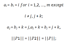
aj and aj+k are the entries for the considered word pair in T1, bj
and bj+k are the corresponding entries for the word pair in T2,
and k is the number of words from wj to wj+k. From the above
assumptions, we have:

Then,

We can also derive the same formula for a sentence pair with only one different word at the kth entry. For the more general
case with a more significant difference in word order or a larger
number of different words, the analytical form of the proposed
metric becomes more complicated (which we do not intend to
present in this paper). The above analysis shows that the sp is a
suitable indication of word order information. sp equals 1 if there
is no word order difference. sp is greater than or equal to 0 if
word order difference is present. Since sp is a function of k, it can
reflect the word order difference and the compactness of a word
pair. The following features of the proposed word order metric
can also be observed:
1. sp can reflect the words shared by two sentences.
2. sp can reflect the order of a pair of the same words in two
sentences. It only indicates the word order, while it is invariant
regardless of the location of the word pair in an individual
sentence.
3. sp is sensitive to the distance between the two words of the
word pair. Its value decreases as the distance increase.
4. For the same number of different words or the same number of
word pairs in a different order, sp is proportional to the sentence
length (number of words); its value increases as the sentence
length increases. This coincides with intuitive knowledge, that is,
two sentences would share more of the same words for a certain
number of different words or different word order if the sentence
length is longer. Therefore, the proposed metric is a good one
[28-31].
Sentence Similarity in Total
Similarity between sentences based on semantic nets is basically
the lexical similarity of sentences. The relationship between
words can be illustrated as word order similarity. This word order
similarity illustrates which word will be there in the summarized
sentence and which words will be there before which words.
The information that is collected in semantic and syntactic way
provides information about the meaning of the sentences.
The similarity between two sentences is modelled as a linear
combination of their semantic similarity and word order similarity.
In equations –

Here the value of δ ≤ 1 decides the relative contributions of
semantic and word order information to the overall similarity
computation. As syntax plays a sub-ordinate role for semantic
processing of text [32], should be a value greater than 0.5, i.e. δ ∈ (0.5, 1].
As a short note we would like to mention that, implementing
this method requires the use of two databases. The first one is
WordNet and the second one is Brown Corpus. WordNet is lexical
database of words that returns similarity issue between two
words. It’s a more like tree hierarchical formation. Starting from
the several roots it will move towards leaf in order to find out
whether words are in same corpus or not. The algorithm then
takes decisions based on this return value [33,34]. The Brown
corpus is also a database of lexical words but it computes the
appearance of words within the corpus using relative frequency:

Here, n = number of times word w occurs in corpus N = number
of words in the corpus
Result
We gave tested in 5 inputs of a Bengali text paragraph for text
summarizing. We have analysis the statistical approach, Sentence
Similarity approach, a result by a random Bengali person. It is
shown below in Table 1.
| Input No |
Size |
Time
(statistical) |
Time (Similarity) |
Time
(Random User) |
Accuracy |
| 1 |
2.2 kb |
0.058 |
10 |
7 |
50% |
| 2 |
3 kb |
0.058 |
13 |
18 |
56% |
| 3 |
4 kb |
0.066 |
22 |
25 |
80% |
| 4 |
11 kb |
0.455 |
100 |
145 |
55% |
| 5 |
23 kb |
0.16 |
325 |
225 |
50% |
Table 1: Text summarizing result.
One of the text summarizing result
Input: A few sentences about greatness of humanity in Bengali,
words counted 70.
Output: Statistical approach A few sentences about greatness of
humanity in Bengali words counted 23.
Output: Sentence Similarity A few sentences about greatness of
humanity in Bengali words counted 6.
Output: A random User A few sentences about greatness of
humanity in Bengali words counted 15.
Analysis:
Comparing both of the algorithm it is clear that both output
illustrates greatness of human being but we look in text words
sentence similarity gives the shortest summarization result but
on the other hand statistical approach gives longest summarizing
result If we take a look at the random user’s output it also points
to the same direction. Analysing just about the output we can say
that both algorithm’s accuracy is about 80 (Figure 2).
Figure 2: Text size / run time analysis
Discussion
While processing the randomized inputs we have seen that most
of the Statistical Approach Summarizer returns the lengthy lines
which contain more information and also in a very short time.
Also, as there is no use of complex algorithms and techniques and
hence processing time is pretty lower for Statistical Approach.
Whenever we read about the output of the statistical approach,
we have seen that it somehow misses some important gist.
Whereas sentence similarity approach mostly does not miss the
gist’s. The sentence similarity takes much more time with respect
to the statistical approach but it returns the less sized line mostly.
And also, it gives a very realistic result. One thing that we have
noticed is with increasing size of text the run time is increasing
almost exponential way for sentence similarity approach whereas
the statistical Approach do not have such characteristics. The
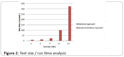
complete timing issue can be shown as the following graph. Text
size and run time analysis is shown in Figure 2.
Above analysis show the text size – run time analysis bar chart.
The slightly blue shades on the graph denote run time of Statistical
Approach. And the red bar denotes the run time for Sentence
Similarity approach.
Accuracy
From the analysis for each of the inputs we are able to see that
both of our approaches at least capable to show the gist’s of
the main content. Reading the output, we can at least gather
an idea that what it is talking about. In statistical analysis we
missed some of the gist’s for Sample Input 5. Whereas sentence
similarity managed to show that gist’s. From this point of view,
sentence similarity is more accurate. Although time complexity of
sentence similarity is a big deal whereas statistical analysis takes
much less time. Apart from that we think that somehow all of our
idea managed to see the daylight.
Conclusion
The sentence similarity-based summarizer is able to give a
satisfactory result for a wide range of documents. The statistical
approach is able to process a large amount data at a very short
time. The sentence similarity approach provides more realistic
result and contains more gist’s than statistical approach. Lack of
Bangla WordNet and Corpus decrease the accuracy of Sentence
similarity approach. Caching of the calculation may also be a
great choice to reduce the run time of Sentence similarity.
References
- Verloren (2002) Wikipedia Data Mining Article.
- Hearst M (2003) What is text mining? Wikipedia Text Mining Article.
- Allen J (1995) Natural Language Understanding. Redwood City, Calif: Benjamin/Cummings 2nd Edition.
- Atkinson J, Mellish C, Aitken S (2004) Combining Information Extraction with Genetic Algorithms for Text Mining. IEEE Intell Syst 19: 22-30.
- Leech, Geoffrey, Smith N (2005) Extending the possibilities of corpus-based research on English in the twentieth century: A prequel to LOB and F-LOB. Int Comput Arch Mod Mediev English 29: 83-98.
- Juan-Manuel Torres-Moreno (2014) Automatic Text Summarization (Cognitive Science and Knowledge Management). ISTE Ltd; Hoboken, NJ: John Wiley & Sons, Inc,1st Edition, 2014.
- Mani I, Maybury TM (1999) Advances in Automatic Text Summarization. The MIT Press, 55 Hayward St. Cambridge, MA, United States, ISBN:978-0-262-13359-3.
- Allahyari M, Pouriyeh S, Assefi M, Safaei S, Trippe ED et al. (2017) Text Summarization Techniques: A Brief Survey. Int J Adv Comput Sci Appl 8: 397-405.
- Kumar YJ, Goh OS, Basiron H, Choon NH, Suppiah PC (2016) A Review on Automatic Text Summarization Approaches. J Comput Sci 12: 178-190.
- AL-Khassawneh YA, Salim N, Jarrah M (2017) Improving Triangle-Graph Based Text Summarization using Hybrid Similarity Function. Indian J Sci Technol 10: 1-15.
- Erkan G, Radev DR (2004) LexRank: Graph-Based Lexical Centrality as Salience in Text Summarization. J Artif Intell Res 22: 457-479.
- Budanitsky A, Hirst G (2001) Semantic Distance in WordNet: An Experimental, Application-Oriented Evaluation of Five Measures. Proceedings at Workshop WordNet and Other Lexical Resources, Second Meeting of the North American Chapter of the Association for Computational Linguistics 27: 1-6.
- Rudrapal D, Das A, Bhattacharya B (2015) Measuring Semantic Similarity for Bengali Tweets Using WordNet. Proceedings of Recent Advances in Natural Language Processing: 537–544.
- Sinha M, Jana A, Dasgupta T, Basu A (2012). A semantic lexicon and similarity measure in Bangla. Proceedings of the 3rd Workshop on Cognitive Aspects of the Lexicon (CogALex-III): 171–182.
- Foltz PW, Kintsch W, Landauer TK (1998) The Measurement of Textual Coherence with Latent Semantic Analysis. Discourse Processes 25: 285-307.
- Jurafsky D, Martin JH (2008) Speech and Language Processing: An Introduction to Natural Language Processing, Computational Linguistics, and Speech Recognition. Prentice Hall: 1-16.
- Ko Y, Park J, Seo J (2004) Improving Text Categorization Using the Importance of Sentences. Inf Process Manag 40: 65-79.
- Kozima H (1994) Computing Lexical Cohesion as a Tool for Text Analysis. Univ Electro Commun: 1-39.
- Landauer TK, Laham D, Rehder B, Schreiner ME (1997) How Well Can Passage Meaning Be Derived without Using Word Order? A Comparison of Latent Semantic Analysis and Humans. Proceedings of 19th Annual Meeting of the Cognitive Science Society: 412- 417.
- Landauer TK, Foltz PW, Laham D (2008) Introduction to Latent Semantic Analysis. Discourse Processes 25: 259- 284.
- Landauer TK, Laham D, Foltz PW (1999) Learning Human-Like Knowledge by Singular Value Decomposition: A Progress Report. Advances in Neural Information Processing Systems 10, Jordan MI, Kearns MJ, Solla SA, eds., Cambridge, Mass : MIT Press 1998 :45-51.
- Li Y, Bandar Z, McLean D (2003) An Approach for Measuring Semantic Similarity Using Multiple Information Sources. IEEE Trans Knowl Data Eng 15: 871-882.
- Liu Y, Zong C (2004) Example-Based Chinese-English MT. Proc 2004, IEEE Int Conf Syst Man Cybern 7: 6093-6096.
- McClelland JL, Kawamoto AH (1986) Mechanisms of Sentence Processing: Assigning Roles to Constituents of Sentences. Parallel Distributed Process 2, Rumelhart DE, McClelland JL and the PDP Research Group, MIT Press 2: 272-325.
- McHale ML (1998) A Comparison of WordNet and Roget’s Taxonomy for Measuring Semantic Similarity. Proceedings of COLING/ACL Workshop Usage of WordNet in Natural Language Processing Systems, 1998.
- Meadow CT, Boyce BR, Kraft DH (2000) Text Information Retrieval Systems, second edition, Academic Press, 2000.
- Michie D (2001) Return of the Imitation Game. Electro Trans Artif Intell 5-B2: 203-221.
- Burgess C, Livesay K, Lund K (1998) Explorations in Context Space: Words, sentences, discourse. Discourse Processes 25: 211-257.
- Charles WG (2000) Contextual Correlates of Meaning. Appl Psycholinguist 21: 505-524.
- Chiang JH, Yu HC (2005) Literature Extraction of Protein Functions Using Sentence Pattern Mining. IEEE Trans Knowl Data Eng 17: 1088-1098.
- Coelho TAS, Calado PP, Souza LV, Ribeiro-Neto B, Muntz R (2004) Image Retrieval Using Multiple Evidence Ranking. IEEE Trans Knowl Data Eng 16: 408-417
- Wiemer-Hastings P (2000) Adding Syntactic Information to LSA. Proceedings of 22nd Annual Conference of the Cognitive Science Society 22: 989-993.
- Hatzivassiloglou V, Klavans JL, E. Eskin E (1999) Detecting Text Similarity over Short Passages: Exploring Linguistic Feature Combinations via Machine Learning. Proceedings of the Joint SIGDAT Conference on Empirical Methods in and National Language Processing and Very Large Corpora, 1999: 203-212.
- Hatzivassiloglou V, Shaw J (1999) Ordering among premodifiers. Proceedings of the 37th Annual meeting of the Association for Computational Linguistics :135-143.




 is a smoothing factor. As
  then the depth of a
word in the semantic nets is not considered. In summary, the
formula for a word similarity measure as:

 is 0:2 and 0:45 [

 is its associated word in
sentence. The use of I (Wi) and
 allows the concerned
two words to contribute to the similarity based on their individual
information contents. Here wi and
 can be calculated as
follows:


