Keywords
Bezier curve, Data fitting, Roots finding
Introduction
Bezier curves [1,2] are widely used in computer graphics to produce smooth curves [3]. The curves are named after the French engineer Pierre Bezier who was an applied mathematician with the car manufacturer Renault. In the early 1960’s, he began searching for ways to automate the process of designing cars. His method has been the basis of the modern field of Computer Aided Geometric Design (CAGD).
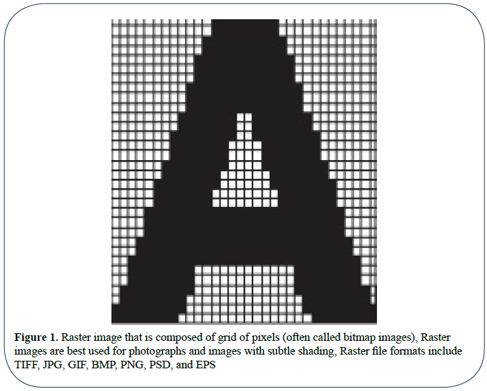
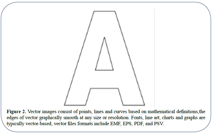
Using Bezier curves changed the common attitude of graphics and introduced the concept of vector graphics as opposed to raster images. A raster image is described in terms of pixels. Each pixel is coded with a color, depending of various algorithm available (jpg, bmp, etc.). The two major problems of raster images is that they are generally big in term of file size and they are not scalable, that means; if you zoom in the image, you will just see the square pixels getting bigger and bigger. In this aspect, Bezier curves are the adopted solution to describe an image in terms of its mathematical representation. The vector graphic file contains the coordinates of some basic points (control points) to describe a series of curves, if the user wants to zoom in, it is only a matter of increasing the space between the control points and it can redraw a perfectly smooth curve again.
Let us describe the difference between Figures 1 and 2:
Figure 1: Raster image that is composed of grid of pixels (often called bitmap images), Raster
images are best used for photographs and images with subtle shading, Raster file formats include
TIFF, JPG, GIF, BMP, PNG, PSD, and EPS
Figure 2: Vector images consist of points, lines and curves based on mathematical definitions,the
edges of vector graphically smooth at any size or resolution. Fonts, line art, charts and graphs are
typically vector-based, vector files formats include EMF, EPS, PDF, and PSV.
In Figure 1, Raster image that is composed of grid of pixels (often called bitmap images), Raster images are best used for photographs and images with subtle shading, Raster file formats include TIFF, JPG, GIF, BMP, PNG, PSD, and EPS.
In Figure 2, Vector images consist of points, lines and curves based on mathematical definitions, the edges of vector graphically smooth at any size or resolution. Fonts, line art, charts and graphs are typically vector-based, vector files formats include EMF, EPS, PDF, and PS.
Bezier curve of degree n
Bezier curve is a parametric curve [4]. Bezier curve of degree n is given as:

Where  , are the control points?
Quadratic bezier curve
The formula of Quadratic Bezier curve is:

Where  are the control points?
Cubic bezier curves
Cubic Bezier curve have three four control points, and has the formula:

Suppose we have a point q(ξ ,η ) . Define a function
 (1)
(1)
Then the problem of finding the shortest distance between the point q(ξ ,η ) and a quadratic Bezier curve is mathematically expressed as follow:
Problem: Find the value  such that:
 (2)
(2)
The value  minimizes the distance between q and the curve B(t) , i.e., B(
 ) is the point located on the curve B(t) which is the closest one to the point q. From (1), it is easily to see that the function f (t) is a polynomial of fourth degree,
 (3)
(3)
Where
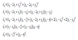
To solve this Problem, we have to find the roots of the equation f ′(t) = 0. Differentiating f(t) given in (3) yields:

Where
 (4)
(4)
As we see is a polynomial of third degree.
Thus, the problem of determining the shortest distance between a point and quadratic Bezier curve is reduced to a problem of finding the roots of a third degree polynomial
There are many methods for finding the roots of the polynomial (4), for example Müller’s method [5].
After determining the real roots of the polynomial P(t), we select only those roots that lie in the interval [0,1] . Let the set of chosen roots be  . Then
  is chosen from the set {
 ,0,1} for which
 (5)
(5)
Algorithm
Inputs 
Compute the coefficients of the polynomial

Deriving f(t) , we get new polynomial

Find the roots of Q3(t) , where its coefficients are determined
Define a set  of real roots that lie in the segment [0,1]
Choose the knot from the set { ,0,1} , such that
If the roots of the polynomial Q3(t) don’t exist in the segment [0,1] , then we choose  that satisfies f (
 ) = min{ f (0), f (1)}
Output 
Numerical Experiments
Test 1
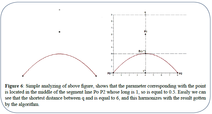
Suppose we want to expert our algorithm in calculating the minimum distance between a point with coordinates (4,9), and quadratic Bezier curve with the control points:  , we run the program of achieved algorithm using Maple [6], we get the value of the parameter t which minimizes distance between the point and the curve mentioned above,
  . Evaluating
  at
at  we get
  ,easily we can conclude that the minimum distance between the point and the curve is the square root of f (t*) , so that it is 6.
Simple analyzing of above figure, shows that the parameter  corresponding with the point B(t*) is located in the middle of the segment line Po P2 whose long is 1, so
  is equal to 0.5. Easily we can see that the shortest distance between q and B(t*) is equal to 6, and this harmonizes with the result gotten by the algorithm.
Test 2
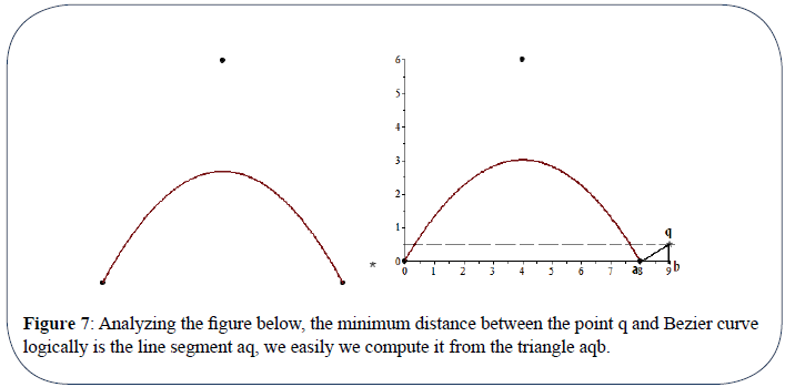
Now we will test the algorithm by choosing new point q(9,0.5) and Bezier curve whose control points are P0 (0,0) P1(4,6) and P2(8,0) .
Running a program of the algorithm gives  =1.008933271 , this value is out of the interval [0, 1]. In this case according to the algorithm we compute f (0) and f (1) ;
  we get f (0) = 81.25 and f (1) =1.25 , then we choose the minimum value of these two values which is 1.25 and so that the minimum distance between the given point and the curve is
Analyzing the above figure, the minimum distance between the point q and Bezier curve logically is the line segment aq, we can easily compute it from the triangle 
So we see that our analyzing does harmonize with the result of the established algorithm.
Test 3
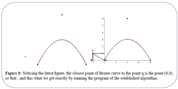
Now if the point is (-2, 1) and the control points of Bezier curve are P0(0,0), P1(4,6) and P2(8,0) in this case we get  = −0.01671531629 , this value doesn’t belong to the interval [0, 1] so we have to compute f(0) and f(1) .
f(0) = 5 And f(1) =101, we have chosen the minimal value 5, so that  = 0 , taking the square root of f(0) = 5 , and so that the minimum distance between the point and the curve in this case is
Noticing the latest figure, the closest point of Bezier curve to the point q is the point (0,0) so that  and we get exactly by running the program of the established algorithm.
Test 4
Let us choose the point  and the control points of Bezier curve are P0 (0,0), P1(4,6) and P2(8,0).
In this case we find that  = 0.833333333 and
  and consequently the minimum distance between the point and the curve is
In this case, noticing the above figure, we can, theoretically, expert our algorithm by computing the parameter  , we first draw the tangent and the line qq* being orthogonal to each other, then the projection of q* on the line segment [0, 1] is
  .
.
 Is close to the value 0.8 on the line segment, and approximately is equal to 0.83. In all cases tests, verify the algorithm does work well (Figures 3-9).
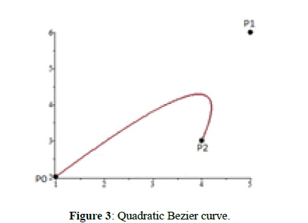
Figure 3: Quadratic Bezier curve.
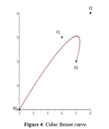
Figure 4: Cubic Bezier curve.
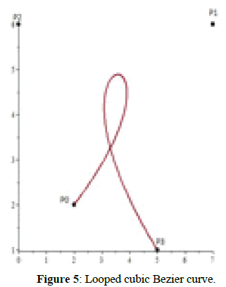
Figure 5: Looped cubic Bezier curve.
Figure 6: Simple analyzing of above figure, shows that the parameter corresponding with the point
is located in the middle of the segment line Po P2 whose long is 1, so is equal to 0.5. Easily we can
see that the shortest distance between q and is equal to 6, and this harmonizes with the result gotten
by the algorithm.
Figure 7: Analyzing the figure below, the minimum distance between the point q and Bezier curve
logically is the line segment aq, we easily we compute it from the triangle aqb.
Figure 8: Noticing the latest figure, the closest point of Bezier curve to the point q is the point (0,0),
so that , and this what we get exactly by running the program of the established algorithm.
Conclusion
This paper presents an improved method for finding the shortest distance between a point and quadratic Bezier curve; this method converts the problem into finding the roots of third degree polynomial, and plays very important role in data fitting using Bezier curves. It is a basic element for curves and surfaces design and for many different fields too. After the theoretic study of algorithm we have changed to write program of it and running it by Maple, we have showed four cases, and analyzed them comparing theoretical solution with programmed one.
References
- Prautsch H, Boehm W, Marco, Paluszuy (2002) Bezier- and B- spline techniques.
- Iqbal K (2013) Fundamental Engineering Optimization Methods.
- Shifrin T (2016) Differential Geometry: A First Course in Curves and Surfaces
- Thomas BG, Thomas Calculus, Massachusetts Institute of Technology.
- Bin Y (2016) Roots of Polynomials (Com S 477/577 Notes).
- Bernardin L, Chin P, DeMarco P, Geddes KO (2011) Maple programming Guide.


 , are the control points?
 are the control points?
 (1)
(1) such that:
 (2)
(2) minimizes the distance between q and the curve B(t) , i.e., B(
 (3)
(3)

 (4)
(4) . Then
  (5)
(5)


 , we run the program of achieved algorithm using Maple [
 . Evaluating
  at
at  ,easily we can conclude that the minimum distance between the point and the curve is the square root of f (t*) , so that it is 6.
 we get f (0) = 81.25 and f (1) =1.25 , then we choose the minimum value of these two values which is 1.25 and so that the minimum distance between the given point and the curve is


 and we get exactly by running the program of the established algorithm.
 and the control points of Bezier curve are P0 (0,0), P1(4,6) and P2(8,0).
 and consequently the minimum distance between the point and the curve is
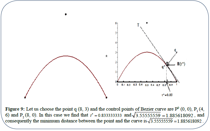
 , and
consequently the minimum distance between the point and the curve is