Keywords
Soil remediation; Analytical model solutions; Electrolysis; Metal removal; CEHIXM process
Introduction
It is necessary to describe the transport and removal of species from solid phase such as soils under the effect of coupled electrichydraulic gradient. Several models have been developed for soil remediation under the action of an electric filed. For examples Probstein and Hicks [1] developed a model for electrokinetic soil remediation. Alshawabkeh and Acar [2,3] developed a generalized theoretical model that describes the reactive solute transport under an electric field. Shapiro and Probstein [4] modeled the removal of contaminants from saturated clay by electroosmosis. Jacobs et al. [5] extended a numerical model for the transport and electrochemical processes for the first time to incorporate complexation and precipitation reactions. Their model confirmed that the isoelectric focusing could be eliminated and high metal removal efficiencies could be achieved by washing the cathode. In all of those studies, the model equations were solved numerically using a linear finite element method. Electrokinetic modeling is based on the applicability of coupled flow phenomena for fluid, solute, current and temperature flow through porous media under the influence of hydraulic, electrical, concentration, and thermal gradients, respectively. The governing equations for these analyses generally have been formulated on the basis of the postulates of irreversible thermodynamics and the applicability of the Onsager reciprocal relations under the assumption of isothermal conditions [6], although equation formulation on the basis of continuity considerations has also been shown in couple of studies [2,3].
The state-of-the-art in modeling electrokinetic remediation is represented by the one-dimensional finite element model for coupled multi-component, multispecies transport under electrical, chemical and hydraulic gradients described in a study conducted by Alshawabkeh and Acar [3]. This study compared the predictions of Pb removal using the model with the results of pilot scale study involving electrokinetic extraction of Pb from a spiked kaolinite sand mixture. A study conducted by Haran et al. [7] developed a mathematical model for decontamination of hexavalent chromium from low surface charged soils. They simulated the concentration profiles for the movement of ionic species under a potential field for different time period. The model predicted the sweep of the alkaline front across the cell due to the transport of OH- ions. A comparison of chromate concentration profiles with experimental data for 28 days of electrolysis showed a good agreement. In order to describe the transport and reaction processes in a porous medium in electrical field, one-dimensional numerical models were developed by several authors [8,9]. In several studies, Choi and Lui [10-13] developed mathematical models for the electrokinetic remediation of contaminated soils assuming the contaminants are mostly heavy metals, water is in excess, the dissociation-association of water into hydrogen and hydroxyl ions is rapid, and that electro-osmosis is significant when compared to electromigration (field-induced transport of ions in an electrolyte as defined earlier) as a transport mechanism. The analytical steady state solutions of electroplating and transport in binary electrolyte arising from electrochemistry were provided in several articles [14-16]. Modified finite difference model of electrokinetic transport in porous media was developed and numerical solutions were provided in couple of studies [8,15].
An assessment of available multispecies transport model and an investigation of long-time behavior of multi-dimensional electrophoretic models were performed by Alshawabkeh and Acar [17]. In a review Shackelford [18] summarized the modeling electrokinetic remediation and emphasized that the prediction of multi-component, multi-species transport with chemical reactions through soil medium represents one of the challenging modeling endeavors in environmental geotechnics. He compared this statement with studies conducted by Acar and Alshawabkeh [19,20] and mentioned that this study provided some insight of the advances along these lines. However, this review stressed on the additional effort that was needed in evaluating the potential limitations in modeling these electrokinetic processes in terms of the assumptions inherent in the models and fieldscale applications. Karim [21] reviewed several other modeling efforts and found that although these studies provide valuable understanding and experience on the modeling of electrokinetic and other similar processes, almost none of them provided any form of analytical solutions as oppose to numerical solutions. Simple particular and trivial analytical solutions of models sometime can provide valuable and close results that can be used in different scenarios. In this study an attempt has been made to provide a simple analytical solution of a model in terms of eigenvalues that can used to describe the contaminant species transport and removal by the CEHIXM processes.
CEHIXM Process
A relatively new in-situ decontamination process namely, CEHIXM was developed at the Cleveland State University, Cleveland, Ohio, USA. This process is able to achieve selective heavy metal decontamination and heavy metal recovery from a background of coarse-grained soil with constituents that are non-toxic but chemically interacting and also present at level that is orders of magnitude higher than the target heavy metals in mass/volume [22]. The CEHIXM process proposes to couple an electric gradient with a suitable hydraulic gradient along with an ion-exchange medium to extract and subsequently recover heavy metal contaminants from soils. A DC electric gradient is used to generate acid by electrolysis of water and a hydraulic gradient is used to pump this acid through the contaminated soil. The circulated acid solution dissolves heavy metals from the soil pores bringing the contaminants into the liquid phase. Khan and Alam [23] discussed the applicability and effectiveness of producing acid solutions by electric gradient. This process also utilizes an ion-exchange medium to remove the extracted heavy metals from the liquid phase. A bench-scale setup of the CEHIXM process was explained in Karim and Khan [22,24]. In brief, the arrangement in the process shows that an electric gradient can be applied across a semi-permeable barrier. The semi-permeable barrier allows the separation of acid generated at the anode from the base generated at the cathode during electrolysis. The acid thus generated is successively pumped through the contaminated soil and an ion-exchange medium by a hydraulic gradient with the intent of dissolving the metal contaminants in the soil and subsequently recovering the metals in the ion-exchanger. Electrolysis is the predominant phenomenon for creating the acid in the anode chamber, and the hydraulic gradient is the primary driving force for transporting the acid through the soil. The electrolysis reactions of the primary electrodes are presented in the following equations:
 (1)
(1)
 (2)
(2)
where, Eo is the standard reduction electrochemical potential. When the H+ rich solution is pumped through the soil sample, containing heavy metals, the acid front facilitates the dissolution of the heavy metal precipitates (hydroxide, carbonate or sulphate, etc.) according to the following reaction:
 (3)
(3)
Thus, free heavy metal cations, Me2+, are generated and move toward the direction of influent flow. This process was successfully used in the bench-scale laboratory studies to remove contaminants from coarse-grained soil. Further details of the process and the experimental results can be found in Karim and Khan [22].
Since CEHIXM is a new process, development of theoretical model is necessary to have a better understanding of species transport and removal mechanisms. The modeling is also required both in an effort to evaluate critically fundamental basis and to develop the necessary design and/or analysis tools in engineering practices. The objective of this article is to present the model formulation and the analytical solution for the CEHIXM process. Predictions using this model were compared with the results of a bench-scale laboratory study involving CEHIXM extraction of lead (Pb), cadmium (Cd), zinc (Zn), and manganese (Mn) from chemically non-interactive solid phase (spent foundry sand with organic content ≈ 0%) and chemically interactive solid phase (a mixture of millpond sludge and spent foundry sand with organic content ≈ 3.5%).
Model Development
Application of electric, hydraulic, chemical and/or thermal gradients to a homogenous medium of soil-water-electrolyte system results in transport of matter and energy. The resulting fluxes of fluid, mass, charge and/or heat through the soil medium, their changes with time and their effects on the properties and composition of the soil medium are significant in various geotechnical/geoenvironmental problems. The various fluxes resulting in the CEHIXM transport process are fluid transport due to a hydraulic gradient, charge transport due to electric gradient, mass transport due to chemical gradient. The one-dimensional differential equation describing transport of N number of chemical species transported under hydraulic, electric and chemical gradients can be represented as follows [3,25]:
 (4)
(4)
For i = 1, 2, 3, …………N.
Where ci(ML-3)=molar concentration of contaminant, Di*(L2T- 1)=effective diffusion coefficient, ui*(L2V-1T-1)=effective ionic mobility, ke(L2V-1T-1)=coefficient of electroosmotic permeability, kh(LT-1)=hydraulic conductivity, E(V)=electric potential, h(L)=hydraulic head, Ri(ML-3T-1)=production rate of the ith aqueous chemical species per unit fluid volume due to chemical reaction such as sorption, precipitation-dissolution, oxidation/reduction, and aqueous phase reactions, and N=number of chemical species.
For the case of nonreactive solute transport (Ri=0), steady state fluid flux (∂h/∂x=constant) and no electrical gradient, Equation (4) becomes;
 (5)
(5)
Usually the advective fluid flux under hydraulic gradients is referred to by the advective velocity (v) that is represented by;
 (6)
(6)
Substituting the advective velocity (Equation 6) into Equation (5), we get;
 (7)
(7)
which is the diffusive-advective solute transport equation widely used to describe nonreactive solute transport.
Customized Model for the CEHIXM Process
In the current study, diffusional coefficient Di * may be assumed to be negligible as the diffusion of cations and anions is very small compared to the flow generated by hydraulic gradients. The absolute values of diffusion coefficients of the representative cations and anions attained under ideal conditions can be found in [25]. The ion mobility of the metals may occur under both electric and chemical gradient. Both ion mobility due to electric and chemical gradients may be assumed to be negligible or absent since the potential gradient is not applied across the soil sample being treated and the chemical gradient is negligible compared to the hydraulic gradient applied. Therefore, the dispersion convection equation can now be simplified and tailored for the use in this study;
 (8)
(8)
The general PDE describing one-dimensional single species transport for the current model is presented as,
 (9)
(9)
Where c is the concentration of the contaminant species, v is the contaminant flow through porous media that follows Darcy’s equation, and R is the rate of dissolution /precipitation of the species. The initial condition is expressed as,
c(x,0)=c0 (10)
For a particular solution, it is assumed that R=0 (for nonreactive solute transport). This assumption is valid for CEHIXM process as the pH of the processing fluid is around 2.0 due to the recirculation of the fluid and most of the metal salts are soluble in that pH. Therefore Equation (9) becomes,
 (11)
(11)
Analytical Solution of the Model
Considering c(x, t)=X(x) T(t) is the solution of Equation (11) [by separation of variables] we get,
 (12a)
(12a)
 (12b)
(12b)
Inserting Equation (12a) and Equation (12b) into Equation (11) we get,

 [dividing by vXT]
 (13)
(13)
where λ is a number (also called a scalar) known as the eigenvalue or characteristic value associated with the eigenvector X or vT. Geometrically, an eigenvector corresponding to a real, nonzero eigenvalue points in a direction that is stretched by the transformation and the eigenvalue is the factor by which it is stretched. If the eigenvalue is negative, the direction is reversed [26]. In this case, no negative eigenvalue is a possibility as the metal concentration is changing with distances from anode towards cathode. Infinite number of solution is possible for the eigenvalue. But, the intent of this study is to find the range of eigenvalue that can fit the experimental data for the CEHIXM process.
From Equation (13) we get,


 (14)
(14)
where, A1 is a constant of integration. Again from Equation (13) we get,


 (15)
(15)
Therefore, typical solution of Equation (11) is
 (16)
(16)
From initial condition (Equation 10) we get,

 (17)
(17)
Therefore, the final form of the analytical solution of the advective equation may be expressed as (rearranging Equation (17),
 (18)
(18)
Equation (18) is valid for both for chemically non-interactive and chemically interactive solid phases and used to generate the analytical data for the concerned metals for the CEHIXM process.
Results and Discussion
The model has been simplified and customized assuming the rate of dissolution/precipitation of the species is zero and/or negligible (R=0, that is nonreactive solute transport). That can be considered valid to some extent for coarse-grained soil/sediment with very low or no organic content. Since the low pH solutions are pumped through the system, precipitation is very unlikely and most the targeted metal salts are fully soluble at low pH. In addition, since no or very negligible organics are present in the soil/sediment, no organometalic complexation will form that will require chelating agent such as EDTA to break the complexation. The primary limitation of this analytical solution is that it may not be used for solid phases that contain high organic materials.
Figures 1 and 2 represent the results of the analytical solutions for the species transport equation (first order hyperbolic) at different eigenvalues, for chemically non-interactive and chemically interactive solid porous media, respectively. Since the experiments were run at v=64.18 cm.hr-1 for chemically non-interactive solid phase and v=25.67 cm.hr-1 for chemically interactive solid phase, the Figures 1 and 2 were developed as a function of time, using Equation (18) based on these two flow velocities, respectively. The experimental flow velocity for both the solid phases was optimized based on the experimental data that can be found in Ref. [22].
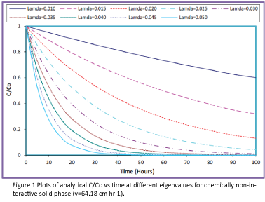
Figure 1: Plots of analytical C/Co vs time at different eigenvalues for chemically non-interactive solid phase (v=64.18 cm hr-1).
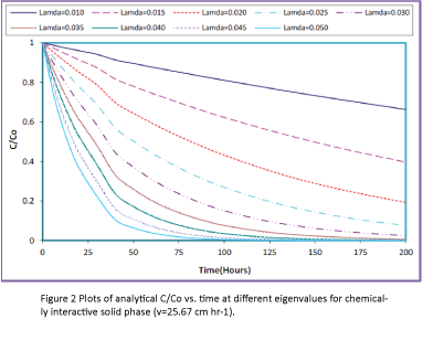
Figure 2: Plots of analytical C/Co vs. time at different eigenvalues for chemically interactive solid phase (v=25.67 cm hr-1).
In order to compare the model results with the experimental data, the experimental data were inserted in Figures 1 and 2 and the new plots were developed. The comparisons of the analytical solutions and the experimental results are presented in Figures 3 and 4 for chemically non-interactive solid phase and Figures 5 and 6 for chemically interactive solid phase.
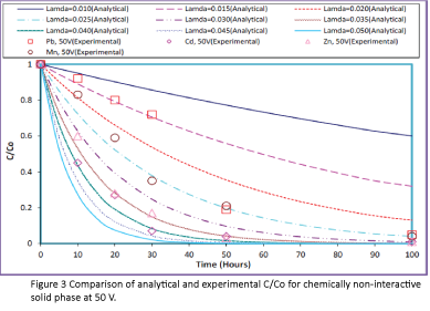
Figure 3: Comparison of analytical and experimental C/Co for chemically non-interactive solid phase at 50 V.

Figure 4: Comparison of analytical and experimental C/Co for chemically non-interactive solid phase at 100 V.
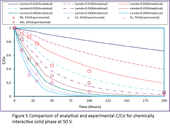
Figure 5: Comparison of analytical and experimental C/Co for chemically interactive solid phase at 50 V.
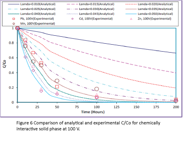
Figure 6: Comparison of analytical and experimental C/Co for chemically interactive solid phase at 100 V.
As seen in Figures 3-7, almost all experimental results fitted within the eigenvalues range of 0.015 to 0.050; however, experimental results for chemically non-interactive solid phase fitted very closely within the eigenvalues range of 0.025 to 0.040 and for chemically interactive solid phase within the eigenvalues range of 0.030 to 0.040. The range of eigenvalues for both the solid phases seems to be similar. Based on the Figures 3-6, the best fit eigen values were extracted and listed in Table 1. It appears that the most likely eigenvalue is approximately 0.020 for Pb, 0.040 for Cd, 0.045 for Zn, and 0.035 for Mn.

Figure 7: Correlations of analytic solutions and experimental data (C/Co).
| Metal |
Chemically non-interactive solid phase |
Chemically interactive solid phase |
Most Likely eigenvalue |
R2 |
| |
(50 V) |
(100 V) |
(50 V) |
(100 V) |
|
|
| Pb |
0.015 |
0.025 |
0.02 |
0.035 |
0.02 |
0.8899 |
| Cd |
0.04 |
0.04 |
0.05 |
0.045 |
0.04 |
0.9918 |
| Zn |
0.035 |
0.045 |
0.045 |
0.045 |
0.045 |
0.9321 |
| Mn |
0.025 |
0.03 |
0.035 |
0.035 |
0.035 |
0.8583 |
Table 1: List of regression coefficients and best fitted eigenvalues.
Conclusion
The C/Co of metals from analytical model predictions agreed very well with the experimental values (C/Co) for Cd and Zn throughout the experiment period. A very good agreement was also observed between the model predictions and the experimental values for Pb and Mn. These agreements occurred within a narrow range of eigenvalues. High correlations between analytical and experimental results demonstrated the validity of the associated equation formalisms and the analytical solutions for the species transport and removal under the effects of coupled electrichydraulic gradient that can used to describe the contaminant species transport and removal by the CEHIXM processes.
References
- Probstein RF, Hicks RE (1993) Removal of contaminants from soils by electric fields. Science 260: 498-503.
- Alshawabkeh AN, Acar YB (1992) Removal of contaminants from soils by electrokinetics: A theoretical treatise. Journal of Environmental Science and Health Part A 27: 1835-1861.
- Alshawabkeh AN, Acar YB (1996) Electrokinetic remediation II: Theoretical model. Journal of Geotechnical Engineering 122: 186- 196.
- Shapiro AP, Probstein RF (1993) Removal of contaminants from saturated clay by electroosmosis. Environmental Science and Technology 27: 283-291.
- Jacobs RA, Sengun MZ, Hicks RE, Probstein RF (1994) Model and experiments on soil remediation by electric fields. Journal of Environmental Science and Health Part A 29: 1933-1955.
- Yeung AT, Mitchell JK (1993) Coupled fluid, electrical and chemical flows in soil. Geotechnique 43: 121-134.
- Haran BS, Popov BN, Zheng G, White RE (1997) Mathematical modeling of hexavalent chromium decontamination from low surface charged soils. Journal of Hazardous materials 55: 93-107.
- Yu JW, Neretnieks I (1996) Modeling of transport and reaction processes in a porous medium in an electrical field. Chemical Engineering Science 51: 4355-4368.
- Segall BA, Bruell CJ (1992) Electroosmotic contaminant-removal processes. Journal of Environmental Engineering 118: 84-100.
- Choi YS, Lui R (1994) Uniqueness of steady-state solutions for an electrochemistry model with multiple species. Journal of differential equations 108: 424-437.
- Choi YS, Lui R (1995) Multi-dimensional electrochemistry model. Archive for rational mechanics and analysis 130: 315-342.
- Choi YS, Lui R (1995) A mathematical model for the electrokinetic remediation of contaminated soil. Journal of hazardous materials 44: 61-75.
- Choi YS, Lui R (1995) Global stability of solutions of an electrochemistry model with multiple species. Journal of differential equations 116: 306-317.
- Choi YS, Yu X (1993) Steady-state solution for electroplating. IMA Journal of applied mathematics 51: 251-267.
- Choi YS, Chan KY (1992) A parabolic equation with nonlocal boundary conditions arising from electrochemistry. Nonlinear Analysis: Theory, Methods and Applications 18: 317-331.
- Choi YS, Chan KY (1992) J Electrodia Chem Interfacial Electrochem 334: 13-23.
- Alshawabkeh N, Acar YB (1994) Presented at the I&EC Special Symposium, the American Chemical Society, Atlanta, GA, pp: 19-21.
- Shackelford CD (1997) Modeling and analysis in environmental geotechnics: An overview of practical applications. In Second International Congress on Environmental Geotechnics 2: 1375-1403.
- Acar YB, Alshawabkeh AN (1996) Electrokinetic remediation I: pilot-scale tests with lead-spiked kaolinite. Journal of Geotechnical Engineering 122: 173-185.
- Acar YB, Alshawabkeh AN (1993) Principles of electrokinetic remediation. Environmental science & technology 27: 2638-2647.
- Karim MA (2014) Electrokinetics and soil decontamination: concepts and overview. Journal of Electrochemical Science and Engineering 4(4): 297-313.
- Karim MA, Khan LI (2001) J Hazard. Mater 81: 83-102.
- Khan LI, Alam MS (1994) Heavy metal removal from soil by coupled electric-hydraulic gradient. Journal of Environmental Engineering 120: 1524-1543.
- Karim MA, Khan LI (2011) Effect of the secondary electrode configuration in removing metal contaminants from soils by the CEHIXM process. Soil and Sediment Contamination: An International Journal 20: 857-875.
- Alshawabkeh N (1994) PhD Dissertation, Louisiana State University, p: 376.
- Burden RL, Faires JD (1993) Numerical analysis.