Keywords
Shock tube-Transient flow simulation-Normal shock wave-CFD
Introduction
Nowadays the usage of Computation Fluid Dynamics in high speed aerodynamics is dramatically increased in
aerodynamic facilities design process. There are many different ways to generate a source of air at a sufficiently
speed and pressure to act as the working fluid of a hypersonic wind tunnel. This includes hotshot tunnels, plasma
jets, shock tubes, shock tunnels, free-piston tunnels, and light gas guns. Various hypersonic wind tunnels have been
constructed at different universities and research centers all over the world. However, these facilities are very costly
and very expensive to run and maintain, the shock tubes are very simple and reasonably low cost to build and
operate. The shock tube is a high speed aerodynamic test facility that enables investigation of moving shock wave
and the loads imposed over a model for high speed flow regimes. To have a pre-view of the flow and moving shock
wave through a shock tube before starting the design process, using the CFD is the best way. Shock tube in its
simplest form is a tube with fixed cross section that is divided by a diaphragm into two areas. After the diaphragm
ruptured, a shock wave proceeds in low pressure area and expansion waves proceed into high pressure area. The conventional process of a normal shock wave traveling and wave diagrams in a simple shock tube are shown in Figure
1. In the present study, the goal is to capture the moving shock wave and the distribution of aerothermodynamics
properties on the wall of tube. Reflected shock wave is not investigated here. There are many practical
investigations on shock tube but numerical simulations are not too many. Daru and Tenaud made a numerical
simulation study on reflected shock wave and laminar boundary layer interaction in a shock tube and defined proper
grid congestion for such a case. They have shown that 4.5 million nodes are sufficient and reliable for such a case
[1]. Al-Falahi et al. developed two dimensional time accurate Euler solver for shock tube applications. In this study,
uniform grid spacing with the number of 356 is used and good results in comparison with practical data were
obtained [2]. All mentioned studies make a good view into flow in shock tubes, but making a fast accurate method
for laminar, ax symmetric flow analysis is not available. In present study, a shock tube can be simulated in a CFD
code very fast and reliable.
Figure 1: Wave diagrams in a simple shock tube
A very important item in numerical simulation of a shock tube is to use proper grid congestion for capturing the thin
layer of moving shock wave. It is also important to generate quadrilateral cells in map form and perpendicular to the
flow direction.
Specifications of test facility
The test facility includes a piston compressor, a pressurized tank, a simple shock tube and three sensors that two of
them are fast response type. the first sensor measures the pressure of behind of the diaphragm and two fast response
sensors duty is to capture the moving shock wave passage. The constant internal diameter of the stainless steel tube
is 67 mm and the total length of tube is 2080 mm and the diaphragm is installed in the 640 mm from the head. The
fast response sensors are located in 15.5 cm and 115.5 cm respectively after diaphragm. There are two sets of tests
and in both the driver gas is dry air. The diaphragms are made of Aluminum foil with the thicknesses of 50 and 80
μm which destruct in 2.7 and 4.8 bar gauge pressure respectively for case1 and 2. Atmospheric conditions are
important for tests, because the low pressure part of shock tube is open to atmosphere and speed of shock wave is a
function of pressure ratio of back and front of diaphragm. The instruction of test facility is shown in Figure 2. It is
important to have the atmospheric condition when running each test. The atmospheric conditions are tracked and
presented in table 1.
Figure 2: Geometry of shock tube of the AUT
Table 1: Initial conditions for simulations
Materials and Methods
Numerical simulation methods
For present research, the conventional Navier Stokes equations in axisymmetric form employed for compressible
gas simulations. Supplementary data are available in reference [3]. The operating fluid considered to be air as a
perfect gas with the vary Cp and thermal conductivity as function of temperature and constant molecular weight.
Viscosity is a function of temperature and modeled by Sutherland's law. Simulations are done in transient mode with
the time step of 1e-05 sec. The pressure-base solver with the Simple mode for pressure-velocity coupling employed
and discretizations for pressure, density, momentum and energy are done in second order.
The assumption of laminar regime is physically true in shock tubes where the duration of test and the Reynolds
number are very low. The initial conditions are the pressure, velocity and temperature for both sides of diaphragm
which is shown in table 1. In this table P is static pressure, V is velocity and T is temperature. Governing equations
consist of conventional continuity, momentum and energy for laminar, adiabatic, axisymmetric flow. For 2D
axisymmetric geometries, the continuity equation can be written as Eq. (1),

Where x is the axial co-ordinate, r is the radial co-ordinate, vx is the axial velocity, vr is the radial velocity andr is
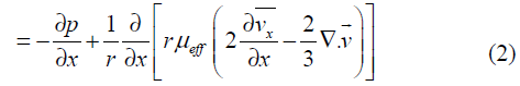
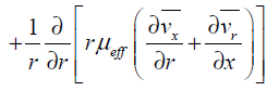
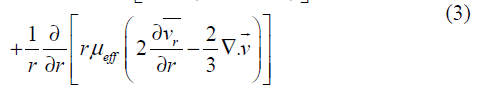
density. For a 2D axisymmetric flow, the axial and radial momentum conservation equations can be written as Eq.
(2) and Eq. (3), respectively.


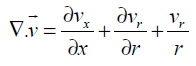
where
 (4)
(4)
In general form, the energy conservation concept can be formulated as Eq. (5),


Where,
 (6)
(6)
For compressible flows, the equation of state (considering ideal-gas concept) can be written as Eq. (7) where R is the
universal gas constant and T is the static temperature.

Grid generation
The domain of simulation is very simple and consists of a tube. Because of the axisymmetric shape of tube, only
half of the model is needed for simulation. Structured quadrilateral grid type is employed for throughout the domain
and the boundary layer grid is generated near wall, so there are 228000 cells in domain. A portion of grid in domain
is shown in Figure 3. To study the grid-independency, two other cases considered for simulation with 900000 cells and
results show no significant variation.
Figure 3: Grid congestion near wall
Results
The practical data extracted from two sensors after the diaphragm only show the time intervals of passing shock. By
using the conventional relations and analytical formulas for shock tubes [4] for 2D, adiabatic and inviscid flow, the velocity of moving shock is definable from ratio of driver gas to driven gas pressure. Table 2 shows the results from
practical tests, simulations and analytical calculations and the results are matched very well. In table 2, t is time
interval for shock to move from sensor 2 location to sensor 3. The data show that the analytical formulas for semi
2D are reliable in constant area circular shock tube.
Table 2: simulation and experimental results
Figure 4 and 5 show the distribution of static pressure along the axis of tube for case1 and 2 for two time intervals.
In case2, pressure ratio in start is higher rather than case1 and the peaks of pressure in shock position is more than
case1 which shows that the shock in case1 is more powerful than case1, also the speed of shock in case2 is more
than case1 as predicted before. As it is shown in Figure 4 and 5, power of the shock waves in time intervals for each
case remains semi-fixed. Figure 6 shows contour of velocity for case1 and 2 when the shock wave is positioned in
the sensor 3 location. It shows that in both cases for specified time, the expansion waves are not reached to the left
wall yet, but it is obvious that in the same shock position, the left wall of tube experiences more pressure drop in
case1. Figures 7 and 8 show the contour of static pressure in three time intervals for case 1 and 2 respectively. The
position of normal shocks and pressure distribution can be tracked. Figure 9 shows the distribution of static
temperature in t=2 msec. As mentioned before, the shock wave in case 2 is more powerful rather than in case 1. The
shock wave in case1 moves faster to the right but the expansion waves are slower move to the left rather than case2.
It is because of the more temperature in front of shock wave and less temperature in front of expansion waves.
However the study of shock wave and boundary layer interactions are not the main goal of present study but the grid
congestion is considered near wall and the Figure 9 shows the velocity vector near wall just before the normal shock
wave.
Figure 4: Distribution of static pressure along axis over wall for case1
Figure 5: Distribution of static pressure along axis over wall for case2
Figure 6: Contour of velocity magnitude
Figure 7: Contour of static pressure (Pa) for case 1
Figure 8: Contour of static pressure for case 2
Figure 9: Boundary layer just before normal shock wave
Figure 10: Distribution of static temperature along axis for case1 and 2 in t=2 msec
Discussion and Conclusion
In present research shock tube of AUT is investigated experimentally and by CFD simulations. Simulation results
show good compatibility to experimental data. It is shown that the power and speed of moving shock wave increases
when the pressure ratio of driver to driven gas increased. Congestion of grid is studied for capturing the shock wave
however for considering the shock wave and boundary layer interactions, a denser grid must be employed. The
represented method can simulate flow in a shock tube very quickly and can be used for design and manufacturing a
new shock tube facility. The location of the sensors can be determined easily. In the practical tests, it is shown that
for capturing the pressure of flow it is necessary to employ ultra high-response pressure transmitter sensors known
as PiezoElectric otherwise the data would not be trustworthy. If the data logger and data capturing systems are
located far from test facility, it is recommended to use ampere transmitters rather than voltage ones. The next step of
present study is to use helium gas instead of air for driver gas to make higher Mach numbers by employing species
equations and modeling shock wave and boundary layer interaction in the presence of model.
References
- V Daru, C Tenaud, Journal of computer and fluids, 2009, Vol. 38, pp. 664-676.
- A Al-Falahi et al., International journal of engineering and applied science, 2010, Vol. 6, No. 5, pp. 320-330.
- T.J Chung, 2002, Computational fluid dynamics,1th ed., Cambridge university press,
- J.D Anderson, 2003, Modern compressible flow with historical perspective, 3th ed., McGraw-Hill,